Data Validation: Limiting Others' Inputs w/o Limiting Your Outputs

Are you ready to learn one of the slickest tricks in Excel? Then read on, my fellow Excelerites! Today we are going to learn about Data Validation.

The overarching goal of Data Validation is to restrict a user to inputting certain items into a cell. For instance, you can restrict the user to only put whole numbers into a cell. 

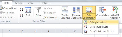
To begin, select the area that you want to restrict. Next, go to the Data tab on your Ribbon and select Data Validation.

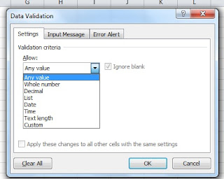
A form will appear. You will notice that it has 3 tabs on it. Under the Settings tab, select the dropdown arrow under Allow.

The default is Any Value. In other words, the user can input any value into the cells. Be adventurous and try experimenting with some of the options. You can start by selecting Whole Numbers. To see if your restriction worked, try inputting a restricted value into your cell. For example, let's say you restrict cell A1 to be only whole numbers between 1-10. If you try to put a 17 in that cell, an error message will appear. 

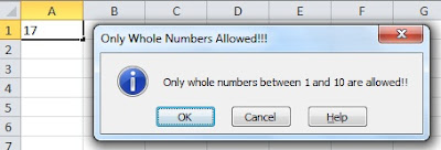
Speaking of error messages, you can customize your error message.Under the Error Alert tab, you can change the error message Style, Title, and Message. Please note that the Style will determine what type of message and restriction is allowed. For instance, the Stop option will not allow any value outside of the restriction. On the other hand, the Information option will. Both, however, will produce a popup. I created the following error message to pop up if the user tries to put a 17 in cell A1. Because I selected the Information option, the user can still change the cell value to 17 but will get this warning before. 

All of this is very easy to learn. Give it a whirl! Stay tuned for next week's post where we delve into the most powerful part of Data Validation: the List!

Extreme Filters & Sorting

This week's tip is one that many of you may already know a bit about. However, we want to take your knowledge one step further and show you some neat functions.

1) Sort by Color: Let's say your boss goes through a list and highlights all the people he wants to meet with in the next week. What is the best way to sort through a list of over 500 employees? Easy, just filter it by color! First create the column filters.

Next, click on the column filter arrow, find the Filter by Color option, and select the color you wish to filter. If your boss selected multiple colors, you can also select the Sort by Color option on that same drop down menu.

2) Custom Sort: Most of your friends probably only know how to use the simple Sort function. However, that tool is very limited. The Custom Sort tool is much more powerful. You will find it on the Home ribbon - Editing - Sort & Filter - Custom Sort

To get started, highlight the table you would like to sort. Make sure you include the headings. Next, select Custom Sort on the Home ribbon. A box like this will appear.

The Sort By drop down will allow you to select which heading or column you want to sort. You can then select what you want to Sort On (usually just Values) and the Order you want it. For this example, We want to sort by ID Number from Smallest to Largest.

You can even add multiple sorting criteria. You do this by clicking on the Add Level button. Now I can first have it sort by ID Number from Smallest to Largest and within that, sort by Last Name from A to Z. That is pretty neat, huh?!

Now you can sort and filter like no one at work can! This is sure to save you time, organize your data more efficiently, and, most importantly, impress your co-workers. Stay tuned for next week's tip!

The Almighty Alt Key

Now that you have mastered the keyboard shortcuts of last week, let's learn how to literally never use your mouse again. Are you ready for this?

Learning the Alt key shortcuts is relatively simple when compared to the shortcuts we outlined last week. The tough part is the growing pains associated with parting with your mouse. Why is it so easy to learn? Because Excel shows you step by step what keys to press. Let's demonstrate.

Let's say we wanted to change the font size or our cell to 14 from 11.

To get started, press the Alt key on your keyboard. You will notice that numbers and letters will appear on your Ribbon (I told you Excel would tell you what to do).

Next, press the "H" key. This will take you to the Home tab. You could have also pressed the "N" or any of the other letters on the Ribbon to take your to the other tabs. Your ribbon should now look like this:

Note that every item on the Ribbon has a letter or number associated with it. To change the font size, just type "FS", type the number 14, and press Enter. That's it!

You may be thinking, "This takes much longer than using my mouse!" However, once you get accustomed to the Alt key and have your favorite functions down, this will save valuable time. In addition, your hands never need to leave the keyboard again! Be adventurous this week and start learning some of your favorite Ribbon functions. Stay tuned for next week's time saving (or awesome) Excel tip!

The Power of the Keyboard Shortcuts

If you wanted to quickly insert a row, how would you go about doing that? If you are like most Excel users, you will use your mouse to click on the row, right click, and then select "Insert Row". What if you wanted to quickly select all items in a column with 203,453 rows? Would you use your mouse to select and scroll allllllllllll the way down?

STOP THE MADNESS!! Never (at least rarely) use your mouse again! This will not only save you precious time but will also amaze your co-workers as they watch you seamlessly navigate your spreadsheet. Using keyboard short cuts will make you look like a competitive ballroom dancer as you glide through Excel. You will make your mouse-using co-workers look like a 16 year old boy at prom.

Here is a great list that summarizes some of the most useful shortcuts. At a minimum, you should learn the following:

• Select entire row = Shift + Spacebar
• Select entire column = CTRL + Spacebar
• Add row (after selection = CTRL + ALT + "+"
• Delete row (after selection) = CTRL + "-"
• Scroll to bottom of list = CTRL + Down Arrow
• Select all items in a list = CTRL + Shift + Down Arrow 

Once you learn those, try embarking on new and exciting keyboard shortcut adventures. For those who are looking for an African Safari, try learning to navigate the Ribbon using the Alt key (stay tuned for a post on this later).

Using keyboard shortcuts will take some time to learn. At first it will seem like it is taking longer than using the trusted mouse, but once you learn them, you will be shocked by how much time they save. Stay strong!